Mathematician Rainer Kress coined a cute name for an insidious kind of triviality: the inverse crime.¹

His usage comes from the study of inverse scattering problems: if you shine light on an object, the light scatters off of it. If you measure the scattered light—the brightness when viewed from different angles—you can reconstruct the object (invert the scattering). The mathematical object that does this is your inverse solver.

The opportunity for crime comes when you test how well your inverse solver works. To do that, you use a forward solver to calculate the scattered light you expect to see for some object (“synthetic data”). Then you run your inverse solver on that synthetic data and see how well the reconstructed object matches the object you started with.

The crime itself is a question of the relationship between your forward and inverse solvers. Kress is concerned about synthetic data that was (or could have been) generated by the forward operator underlying or implied by the inverse solver. In such a case, it’s no surprise when inversion appears successful. From another perspective, if the two solvers are equivalent in some sense—they implicitly or explicitly use the same ideas, they assume the same things, they approximate to the same order, they share code—one could accuse you of some degree of inverse crime.

In the worst case, if the relationship between the forward and inverse solvers is trivial inversion, then you’re not testing whether your inverse solver is correct. You’re testing whether it’s a correct implementation of undoing the forward solver’s operations step by step.

Inverse crimes vary just as do degrees and senses in which the forward and inverse solvers are connected. What they have in common, and what distinguishes them from non-criminal cases, is that your validation method can’t give you all the information you want about correctness—and it invites you to fool yourself about it.

Examples

Inverse crimes concern synthetic data and validation in general, not just in scattering problems.

One trivial inversion occurs when, to unit test a method f, you run f(2) to get an answer (2.571) and then add @test f(2) == 2.571 to your test suite. That’ll catch a change in f’s behavior, but is it the right behavior?

Or if your test suite passes @test f(g(x)) == x for various values of x, then you’ve validated only that f inverts g. That’s meaningful, but you still can’t say that either function does what you want.

These are easy to spot and relatively easily fixed, but crimes are often subtle! You may not think of your tests as inverting anything, and a moral equivalence can be buried deep.

In machine learning, training on the test set can be viewed as an inverse crime. Even iterating on a model to get better performance on the test set falls under the shadow, along with a number of other surreptitious or accidental ways of accomplishing the same thing.

Problems of doublecounting evidence or confirmation bias can be cast in terms of inversion.

(Nontriviality can also be subtle. If you want to invert f(x) = x^2, you have two possible solutions. If your inverse solver picks out one, that’s informative in a way that may require interpretation. Wirgin (2004) elaborates on the subject.)²

In depth: Curve fitting for filter characterization

Here’s a trickier and more realistic case. I want to fit transmission spectra of some filters—say, transmitted power as a function of frequency for optical ring resonators in a notch (or “all-pass”) configuration. There’s no real lesson at the end of this—it’s more of an exercise in thinking about model validation.

First attempt: Trivial inversion

I remember that the energy of a resonator decays exponentially in time, so it should have a Lorentzian lineshape in the frequency domain. With a little reasoning about special cases I can guess a specific functional form, and write a method to fit the parameters to some data.

using Optim
using Zygote
using GLMakie

function power_transmission_spectrum(ω, # frequency
        ω_0, # resonant frequency
        κ_i, # intrinsic loss
        κ_e) # extrinsic loss
    return 1 - κ_i * κ_e / ((ω - ω_0)^2 + ((κ_i + κ_e)/2)^2)
end

function fit_transmission(ωs, data, p_0)
    loss(p) = sum(abs2.(
        power_transmission_spectrum.(ωs, p...) .- data))
    g!(G, p) = (G .= loss'(p)) #'# silly syntax highlighter
    h!(H, p) = (H .= hessian(loss, p))
    result = optimize(loss, g!, h!, p_0)
end

This should approximate my devices pretty well, but I’d like to see some evidence. I could generate synthetic data the easy way, by adding noise to the transmission function I already wrote:

function synthesize_data(ωs, p, noise_amplitude=0.1)
    return power_transmission_spectrum.(ωs, p...) .+ 
        noise_amplitude*randn(length(ωs))
end

ωs = range(-0.5, 0.5, length=1000)
p_true = [0.1, 0.05, 0.02]
data = synthesize_data(ωs, p_true)
result = fit_transmission(ωs, data,
    [ωs[argmin(data)], 0.01, 0.01])

julia> result.minimizer
3-element Vector{Float64}:
 0.10094963595329196
 0.01968074906926952
 0.051693643609924414
julia> fig, ax = scatter(ωs, data, color=:darkblue);
julia> ax.xlabel = "δω";
julia> ax.ylabel = "Normalized transmitted power";
julia> lines!(ωs, power_transmission_spectrum.(ωs,
    result.minimizer...), color=:red, linewidth=5);
julia> current_figure()

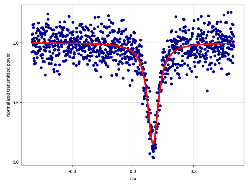The test helpfully reminds me that my transmission formula is symmetric in the intrinsic and extrinsic loss.^{a a} In fact, if I had used a gradient-only method, the fit could have gotten stuck at a saddle point with the two losses equal. ⏎ That’s important for interpreting results, so at some point I’ll have to think of another way of distinguishing the two.

Still, this isn’t the test I really wanted. It tests whether optimize inverts adding noise to the transmission spectrum. Or, no, whether optimize inverts adding noise to my specific single implementation power_transmission_spectrum. If my calculation of the transmission spectrum is a bad approximation, or if I made a typo and it’s entirely wrong, I’ll never know.

Second attempt: Disguised inversion

Well, maybe I should come up with a different way to generate test data. I remember that resonators can be modeled like RLC circuits, so I can find the resistance, inductance, and capacitance corresponding to my Lorentzian parameters, then put that circuit into a SPICE simulator or something entirely disconnected from my code.

That strategy’s well-intentioned, but it’s still a crime, as it turns out. Sure, it’s less egregious, but the RLC circuit isn’t another independent way of modeling an ideal resonator—it’s exactly equivalent to the Lorentzian in the sense that matters. The parameters R, L, and C (scaled to an input/output impedance Z_0) contain the same information as ω_0, κ_e, and κ_i. The approximation to the underlying physical process is identical. It’s possible I’ll catch implementation bugs, but that’s not enough. I want to test how good that approximation is.

Third attempt: Physical derivation

To do this, we had best understand where the approximation comes from.^{b b} For some problems, you can get away without understanding if you get your hands on calibration standards or datasets. ⏎ Light in an input waveguide passes by the ring with some light coupling into the ring and circulating, accumulating phase $\varphi$ with each round trip. The circulating amplitude $α$ decays over time $(a),$ radiating away or bouncing off of imperfections in the ring. It also couples back into the waveguide with each round trip $(k),$ interfering with the input light that passed through $(r).$ We can solve for the amplitude in the ring in the steady state, and it looks like this:

$$\begin{align} \alpha &= \alpha_{\text{in}} k + \alpha_{\text{in}} k (ra\, e^{-i φ}) + \alpha_{\text{in}} k (ra\, e^{-i φ})^2 + ... \notag\\ &= \frac{\alpha_{\text{in}} k }{1 - ra\, e^{-i φ}}\notag\\ \alpha_\text{out} &= \alpha_\text{in} r - \alpha k \notag\\ \frac{\alpha_\text{out}}{\alpha_\text{in}} &= r - \frac{k^2}{1 - ra\, e^{-i φ}} \notag\\ &= e^{-iφ}\frac{r - r^2a - (1-r^2)e^{iφ}}{1-ra\, e^{-iφ}}\notag\\ &= e^{-iφ}\frac{(a-1)(1-r^2) -a + r\, e^{iφ}}{1-ra\, e^{-iφ}} \\ \left\lvert\frac{\alpha_\text{out}}{\alpha_\text{in}}\right\rvert^2 &\approx \frac{r^2 + a^2 - 2ra\cos φ}{1 + (ra)^2 - 2ra\cos φ} \end{align}$$ We’ve already made a couple assumptions: that $k^2 = 1 - r^2$ (there’s no loss in the coupler), and that $(1-a)(1-r^2) \ll a .$ We might use either Eqn. 1 or 2 to generate synthetic data.

Technical note: How do you get to the Lorentzian?

Resonance occurs when the denominator is minimized, at $\cos φ = 1$ or $φ~=~2π n$ for integer $n$ . We can expand in small $\delta φ$ around that value: $$\begin{align*} \left\lvert\frac{\alpha_\text{out}}{\alpha_\text{in}}\right\rvert^2 &\approx \frac{(r - a)^2 + ra\,\delta φ^2}{(1 - ra)^2 + ra\,\delta φ^2} \\ &= 1 - \frac{(1 - r^2)(1 - a^2)}{(1 - ra)^2 + ra\,\delta φ^2}. \end{align*}$$ If we define $k_1 = \frac{(1+r)(1-a)}{\sqrt{ra}}, k_2 = \frac{(1-r)(1+a)}{\sqrt{ra}}$ , then

This is the functional form we wanted, but $k_1, k_2$ don’t correspond to the intrinsic and extrinsic $\kappa_i, \kappa_e .$ In fact, if we want $\kappa_i \propto 1-a^2$ and $\kappa_e \propto 1-r^2,$ then

$$\begin{align*} \left\lvert\frac{a_\text{out}}{a_\text{in}}\right\rvert^2 &\approx 1 - \frac{\kappa_i \kappa_e}{\big(\frac{\sqrt{ra}}{(r+a)/2}\frac{\kappa_i+\kappa_e}{2}\big)^2 + \delta \omega^2}. \end{align*}$$ So above I accidentally included an implicit approximation that gets worse the more different $a$ and $r$ are (the more different their arithmetic and geometric mean, or the further the device from critical coupling).^{c c} This is characteristic of Fabry Pérot resonators, where the “natural” Lorentzian lineshape due to exponential decay gets modified because the extrinsic coupling is presented to a circulating wave only periodically, not continuously. The exact expression should be expressible as a sum of Lorentzians that’s been named after George Biddell Airy, although it’s not the well-known Airy function. Unfortunately I can’t point to a source that goes to the trouble for the ring resonator case, but it’s somewhere between a Lorentzian and the discrete Fourier transform of a uniformly sampled exponential decay, I suppose. ⏎ I certainly wasn’t testing that before. How much does that matter, and how would I correct for it?

Why approximate at all?

Why don’t I just use the more accurate Eqn. 2 for my model? Sometimes that’s the best option. (One can even test it using synthetic data from an approximate model.) In this case, it’s kind of annoying, because $\varphi$ is a strange parameter. The ring resonator supports many resonances periodic in frequency.^{d d} This period is known as the free spectral range (FSR). Sometimes you care more about the ratio of FSR to linewidth than about the linewidth (or quality factor) itself, in which case you may still want to determine FSR independently rather than use the realistic model. ⏎ Using $\varphi$ in my parameterization forces me to pick one out, but I don’t really care which one it is. In other words, for my purposes, $\varphi$ is effectively two parameters, $\delta\varphi$ and $n,$ the integer multiple used to satisfy the resonance condition. If I want, and if I’ve thought carefully about what it means, can’t I choose $n$ arbitrarily? Then I have another 3-parameter model that shouldn’t give me any more trouble than the Lorentzian. But I really do care about $\kappa_i$ more than the round-trip amplitude decay. The connection between $a, r,$ and $\kappa_1, \kappa_2$ depends on physical attributes of the filter (length and effective index) that I don’t necessarily know but would effectively be assuming by choosing $n.$ It’s probably better to abstract all that away.

Other details

Once I encounter real data, I might find there are other details I have to account for to extract the information I want. Uneven background transmission, optical nonlinearities, photodetector dark counts, various sources of noise. Some details might be calibrated or otherwise preprocessed away, others might need to be part of my model. I’m probably not going to be able to keep my model innocent of feedback from its output; instead, I’ll have to adjust it based on how I judge its fit to the data. That doesn’t compromise the experiment, but it is one way confirmation bias creeps in. Keeping synthetic test data “physical” and out of the range of the model is one line of defense.